Big O, code efficiency analysis
16 min read


Andrei Chirila
@chirila_In this article I would do my best to introduce you to algorithmic complexity and a way to roughly measure it by using the Big O notation.
Why measuring code efficiency is important
First of, probably the most significant fact to why it is important, is because we want to reason about how the code we currently have affects our programs. We can test our code on a smaller scale, but how are we going to predict the way our code is going to run on a bigger scale and how the code we write is able to solve a problem of a particular size.
Second reason, would be to understand how the code we write, when we design or implement an algorithm would affect the problem at hand. You can start taking decisions based on how certain data structures, or implementation details can impact the final time complexity of our program.
Why should we care
One argument that is usually given, on why you shouldn't care about it, is that computers are getting progressively faster, thus making the computations faster. But on the other hand, the data volume that is being computed gets bigger and bigger, to the point that in 2016 google announced that they are serving 130.000.000.000.000 (130 trillion) pages, compared to their report from 2013 when they only served around 30.000.000.000.000 (30 trillion). While computers getting faster is undoubtedly true, we can see how the data volume we are working with gets massive, so writing just a simple algorithm that goes over the whole data set isn't enough, even today.
Pre requirements
To follow along with this article it would be advised to have some previews knowledge on the following:
- basic understanding of algorithms
- basic understanding of computer science fundamentals
- basic understanding of data structures
Code analysis
Now that we understand why writing efficient code matters, let's talk about what makes our code efficient and how do we measure the complexity of an algorithm.
We can measure an algorithm complexity by:
- time (duration)
- space (memory)
With this in mind, there comes a big problem, how do we generalize and abstract these measurements. If we are talking about time complexity, how do we measure the time our program takes to execute a piece of code. We can definitely use timers to find out, which would be the intuitive way of doing it, in node we can simply record the time before and after the execution and subtract those values:
function average(nums) {
  let total = 0;
  for(let i = 0; i < nums.length; i++) {
    total += nums[i];
  }
  return total / nums.length;
};

const start = new Date();
average([23, 51, 88, 49, 90, 7, 64, 77, 12, 8, 96]);
const end = new Date();

console.log(`Execution time: ${end - start}ms`);
Doing it this particular way, exposes our measurements to inconsistency:
- execution time, varies between algorithms
- execution time, varies between implementations
- execution time, varies between systems/computers
- execution time, is not predictable on lager scale
In order to consistently measure an algorithm we need a better alternative, that can:
- count the amount of operations we perform without worrying of implementation details
- focus on how the time and space complexities scale
- measure the algorithm based on the size of the input and the number of steps taken
Growth of operations
Let's look at a code example, that will iterate over a list of elements and return whether or not an element exists within the list:
function find(list, element) {
  for(let i = 0; i < list.length; i++) {
    if(list[i] === element) return true;
  }
  return false
};
In this scenario, what is the time complexity of our code ? Well, it depends on how lucky you are. It could be that the first element in the list is our element, in that case it only goes over the loop once, and it's done, this is known as best case scenario. But it can as well be that our element isn't within the list, in that case we have to go through the entire list and return false, which is the worst case scenario. We can also run multiple examples on this code and see how many iterations it goes through, and that will give us the average case, on average we are likely to look at half of the list to find our element.
Asymptotic Notations
Asymptotic notations are mathematical tools used to represent the complexities of algorithms. There are three notations that are commonly used:
Big Omega (Ω) Notation, gives a lower bound of an algorithm (best case)Big Theta (Θ) Notation, gives an exact bound of an algorithm (average case)Big Oh (O) Notation, gives an upper bound of an algorithm (worst case)
Sometimes is useful to look at the average case to give you a rough sense of how the algorithm will perform in the long run, but when we talk about code analysis we usually talk about worst case, because it usually defines the bottleneck we are after.
Big O Notation
Let's look at the example from before, that computes the average of a given list of numbers, and specifically at this line:
function average(nums) {
  let total = 0;
+  for(let i = 0; i < nums.length; i++) {
    total += nums[i];
  }
  return total / nums.length;
};

average([23, 51, 88]);
We right away notice a loop which goes from a starting point of i = 0 to the i < nums.length, meaning that the time complexity of this code would be the size of the given input nums, in this case having a length of 3 (elements in the list of nums). We can generalize the input name as n. Therefor we can say the complexity of our average function is O(3n), furthermore we can drop any coefficients and constants and we are left with a complexity of O(n).
At this point you might wonder how are we able to drop that 3; that's just a simplification we make which is possible because Big O is only interested in how the performance of our algorithm changes in relation with the size of the input.
Simplifications
Let's look at some example simplifications to better understand how we can simplify our notation.
- O(6 * n) = O(n)
- O(14n) = O(14 * n) = O(n)
- O(3891n) = O(3891 * n) = O(n)
- O(n / 4) = O(¼ * n) = O(n)
- O(3n * n * 322) = O(n * n) = O(n2)
- O(n2 + 2n + 9) = O(n2)
- O(800 + n + n3 + n2) = O(n3)
- O(4n12 + 2n) = O(2n)
- O(441) = O(1)
Now that we have seen some examples we can go ahead and define some rules:
Law of Multiplication
- used with
nestedstatementsWhen Big O is the product of multiple terms, we can drop any coefficients and constants
Law of Addition
- used with
sequentialstatementsWhen Big O is the sum of multiple terms, we can keep the largest term, and drop the rest
Time complexity analysis examples
To better understand how we can analyze the time complexity of our code and simplify our notation let's look at some trivial examples.
// We have 2 separate loops
// O(3n + 3n) = O(n) -> addition, we keep the largest term
function exampleOne(n) {
  for(let i = 0; i < n.length; i++) {
    // code
  }
  for(let j = n.length - 1; j > 0; i--) {
    // code
  }
};
// calling the function with [1, 2, 3] -> list of length 3
exampleOne([1, 2, 3])

// We have 2 separate loops, one of them being a nested loop
// O(5n * 5n + n / 2) = O(n² + n) = O(n²) -> addition, we keep the largest term
function exampleTwo(n) {
  for(let i = 0; i < n.length; i++) {
    for(let j = 0; j < n.length; j++) {
      // code
    }
  }
  for(let k = n.length / 2; k > 0; k--) {
    // code
  }
};
// calling the function with [5, 6, 7, 8, 9] -> list of length 5
exampleTwo([5, 6, 7, 8, 9])

// First outer loop, iterates a constant number of times (100), and has a nested loop
// Second loop, iterates a constant number of times (4350)
// O(100 * 4n + 4350) = O(n) -> addition, we keep the largest term
function exampleThree(n) {
  for(let i = 0; i < 100; i++) {
    for(let j = 0; j < n.length; j++) {
      // code
    }
  }
  for(let k = 0; k < 4350; k++) {
    // code
  }
};
// calling the function with [2, 4, 6, 8] -> list of length 4
exampleThree([2, 4, 6, 8])
Space complexity analysis examples
Until now we only talked about time but space is equally important depending on the specifications of our system. It might be the case that we have a limited memory and thus we would have to make some time complexity tradeoffs in order to gain some better space complexity.
// 3 variables created that are not dependent of the input size
// O(3) = O(1) -> simplification of a constant term
function average(list) {
  // declaring a variable 'total'
  let total = 0;
  // declaring a variable 'i' once
  for(let i = 0; i < list.length; i++) {
    /**
    Even though we create this variable every loop
    at the end of each iteration it will be disposed
    so we only ever have one variable
    */
    const current = list[i]
    total += current;
  }
  return total / list.length;
};

// 3 variables created, one grows with the input size
// O(2 + n) = O(n) -> addition, we keep the largest term
function reverse(list) {
  // variable grows with the input size
  const reversedList = [];

  for(let i = list.length - 1; i >= 0; i--) {
    const current = list[i];
    // pushing each element in the list in the 'reversedList' thus growing it's size
    reversedList.push(current);
  }
}
Complexity classes
There are a set of complexity classes that we will go over in an ascending order from most performant to least performant ones.

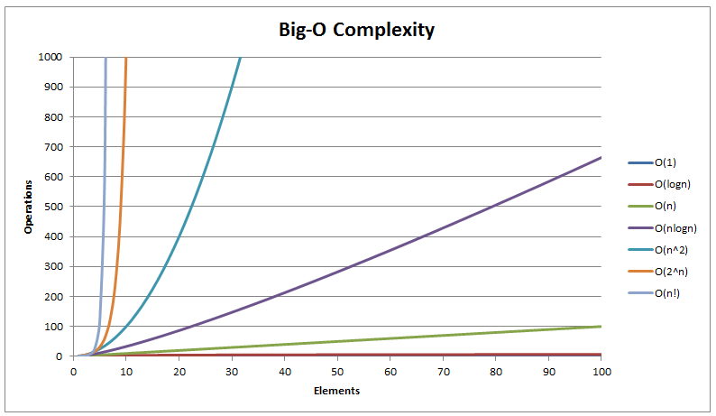
Let's have a look on how these classes would scale with the input size;
| Complexity Class | n= 10 | n= 100 | n= 1000 | n= 1000000 |
|---|---|---|---|---|
| O(1) | 1 | 1 | 1 | 1 |
| O(log n) | 1 | 2 | 3 | 6 |
| O(n) | 10 | 100 | 1000 | 1000000 |
| O(n log(n)) | 10 | 200 | 3000 | 6000000 |
| O(n²) | 100 | 10000 | 1000000 | 1000000000000 |
| O(2ⁿ) | 1024 | 1267650600228229401496703205376 | Have fun! | Have fun! |
Constant – O(1)
- amount of time or steps it takes does not depend on the input size
- can have loops or recursive functions as long as the number of iteration or calls are independent of the input size
When we want to identify constant time we usually look for operations that aren't growing/scaling with the input size, typically code that doesn't iterate over the size of the input. Some operations that we consider to run in constant time are: arithmetic operations, accessing an array index, hashmap lookups, inserting a node into a linked list.
// Time: O(1) -> does not depend on the input size
// Space: O(1) -> does not grow with the input
function isEven(n) {
  let result;
  if(n % 2) {
    result = false;
  } else {
    result = true;
  }
  return result;
}

// Time: O(1)
// Space: O(1)
function sumFirstAndLast(list) {
  // accessing array index and getting it's length is a constant operation
  const result = list[0] + list[list.length - 1];
  return result;
}
Logarithmic – O(log(n))
- amount of time or steps it takes grows as a logarithm of the input size
To better understand what this means, we need to understand what a logarithm is, in short a logarithm is the opposite of an exponent. If in the case of an exponent we multiply, in the case of a logarithm we divide
Exponent
- 24 = 16 – 2 * 2 * 2 * 2
- we say 2 to the power of 4 is 16
Logarithm
- log216 = 4 – 16 / 2 = 8 / 2 = 4 / 2 = 2 / 2 = 1
- we count how many times (4 times) we divided by 2 which is our base
- we say log in base 2 of 16 is 4
Some algorithms that have log complexity are binary search and bisection search
// Time: O(log(n)) -> each iteration we divide by 2
// Space: O(1)
function countDownStep(n, step = 2) {
  for(let i = n; i > 0; i /= step) {
    console.log(i);
  }
}

// Binary search of a list
// Time: O(log(n)) -> each iteration we divide our list by 2
// Space: O(1)
function indexOf(list, element) {
  let start = 0;
  let end = list.length - 1;

  while(start <= end) {
    let mid = Math.floor((start + end) / 2);
    // if element is at the middle we return it's index
    if(list[mid] === element) return mid;
    // going either right or left of the list
    if(list[mid] < element) {
      start = mid + 1;
    } else {
      end = mid - 1;
    }
  }
  return -1;
}
Linear – O(n)
- amount of time or steps it takes depends on the size of the input
- iterative loops and recursive functions
We have seen a lot of linear iterative complexity at this point, so let's jump into some examples where I would include an iterative and recursive linear complexity example (if you are not familiar with recursion I would advice to research it, will write an article about it at some point and link it here).
// Iterative factorial
// Time: O(n) -> iterating n times
// Space: O(1)
function iterFactorial(n) {
  let product = 1;
  for(let i = 1; i <= n; i++) {
    product *= i;
  }
  return product;
}

// Recursive factorial
// Time: O(n) -> number of function calls is dependent of n
// Space: O(n) -> there are always n function calls in our call stack
function recurFactorial(n) {
  // base case
  if(n <= 1) return 1;

  return n * recurFactorial(n - 1);
}
If you were to time these 2 functions, you may notice that the recursive one runs slower then the iterative version, due to the function calls. You can optimize it using a memoization strategy, but I would talk about this in another article.
Linearithmic – O(n log(n))
- amount of time or steps it takes depends on the size of the input that grows logarithmic
- sequential loops nested in log complexity loops
Linearithmic complexity is also known as loglinear or n log n, this particular complexity class is bigger than O(n) but smaller than O(n2). Many practical algorithms are linearithmic, most commonly used being merge sort and quick sort.
// Time: O(n log(n)) -> sequential loop (slice method), nested into log loop
// Space: O(1)
function iterPrintHalf(str) {
  for(let i = str.length; i >= 1; i /= 2) {
    const result = str.slice(0, i);
    console.log(result);
  }
}

// Time: O(n log(n)) -> sequential loop (slice method), into log recursive call
// Space: O(n) -> there are always n size function calls in our call stack
function recurPrintHalf(str) {
  console.log(str);
  if(str.length <= 1) return;

  const mid = Math.floor(str.length / 2);
  const result = str.slice(0, mid);

  return recurPrintHalf(result);
}
Polynominal – O(nc)
- n being the size of input and c being a constant, where
c > 1 - typically multiple nested loops or recursive calls
- includes quadratic O(n2), cubic O(n3)
Most of the polynominal algorithms are quadratic and include bubble sort, insertion sort, selection sort, traversing 2D arrays
// Time: O(n²) -> 2 nested loops
// Space: O(1)
function bubbleSort(list) {
  for (let i = 0; i < list.length; i++) {
    let temp1 = list[i];

    for (let j = i + 1; j < list.length; j++) {
      let temp2 = list[j];

      if(temp1 > temp2) {
        // swap
        list[i] = temp1;
        list[j] = temp2;
        // update
        temp1 = list[i];
        temp2 = list[j];
      }
    }
  }
  return list;
}
Exponential – O(cn)
- n being the size of input and c being a constant, where
c > 1 - recursive functions, where more than one call is made for each size of the input
Many important problems are exponential by nature but as cost can be high it leads us to consider more approximate solutions as they provide better time complexities. Some exponential algorithms include towers of hanoi, recursive fibonacci
// Time: O(2ⁿ) -> two recursive calls are made for each input
// Space: O(n) -> we only have n calls on the call stack
function fibonacci(n) {
  if(n === 0) return 0;
  if(n === 1) return 1;

  return fibonacci(n - 1) + fibonacci(n - 2);
}
This recursive function can be optimized by using a memoization strategy.
Factorial – O(n!)
- recursive functions, where each call is dependent on the input size
The main difference between exponential and factorial is that in exponential we make a constant number of recursive calls, where in factorial we are making n number calls. Popular algorithms that are factorial include traveling salesman, permutations
// Time: O(n!) -> n recursive calls are made based on the size of the input
// Space: O(n) -> we only have n calls on the call stack
function trivialExample(n) {
  if(n === 1) return 1;
  // code

  for(let i = 0; i < n; i++) {
    trivialExample(n);
  }
}

// Time: O(n!) -> n recursive calls are made based on the size of the input
// Space: O(n) -> we only have n calls on the call stack
function permutations(string, char = "") {
  if(string.length <= 1) return [char + string];

  return Array.from(string).reduce((result, char, idx) => {
    const reminder = string.slice(0, idx) + string.slice(idx + 1);
    result = result.concat(permutations(reminder, char));
    return result;
  }, []);
}
Conclusion
We talked about why writing efficient code is important and what are some strategies we can take to measure our code efficiency. We introduced Big O Notation as a solution to generally analyze the complexities of our algorithms, and briefly mentioned the other 2 asymptotic notations. We then analyzed some code using Big O notation, and talked about the most used complexity classes and how are they scaling with the input size, giving examples to better visualize and understand the way we typically analyze our code.